Polynomial Loc-Scale-Regression

Setup and Imports

import jax
import jax.numpy as jnp
import liesel.goose as gs
import liesel.model as lsl
import numpy as np
import pandas as pd
import plotnine as p9
import tensorflow_probability.substrates.jax.distributions as tfd

import liesel_gam as gam

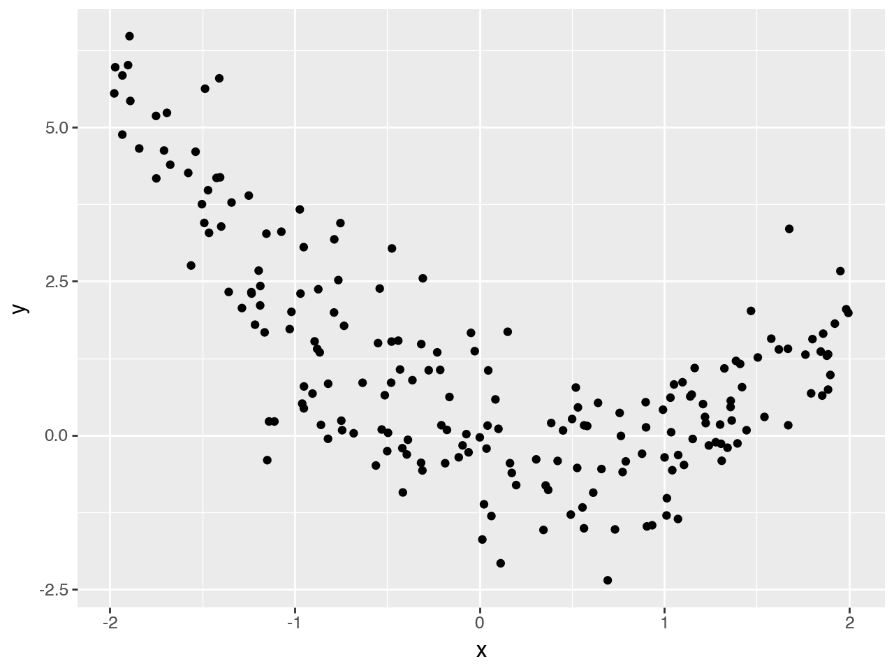
rng = np.random.default_rng(1)
x = rng.uniform(-2, 2, 200)

log_sigma = -0.2 * x
mu = -x + x**2
y = mu + jnp.exp(log_sigma) * rng.normal(0.0, 1.0, 200)

df = pd.DataFrame({"y": y, "x": x})

(p9.ggplot(df) + p9.geom_point(p9.aes("x", "y")))

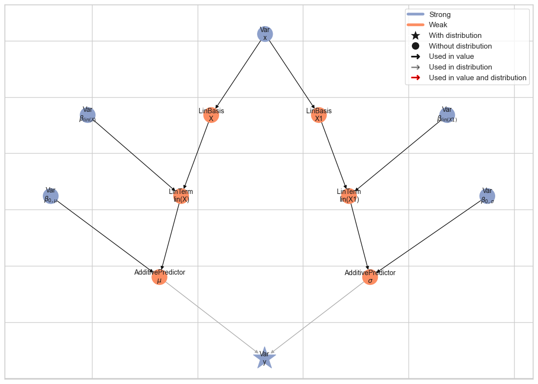
Model Definition

loc = gam.AdditivePredictor("$\\mu$")
scale = gam.AdditivePredictor("$\\sigma$", inv_link=jnp.exp)


y = lsl.Var.new_obs(
    value=df.y.to_numpy(),
    distribution=lsl.Dist(tfd.Normal, loc=loc, scale=scale),
    name="y",
)

tb = gam.TermBuilder.from_df(df)

loc += tb.lin("x + {x**2}")
scale += tb.lin("x")

Build and plot model

model = lsl.Model([y])
model.plot_vars()

Run MCMC

Since we used the inference arguments to specify MCMC kernels for all parameters above, we can quickly set up the MCMC engine with gs.LieselMCMC (new in v0.4.0).

eb = gs.LieselMCMC(model).get_engine_builder(seed=1, num_chains=4)

eb.add_burnin(1000)
eb.add_posterior(10_000, thinning=10)

engine = eb.build()
engine.sample_all_epochs()
results = engine.get_results()

liesel.goose.builder - WARNING - No jitter functions provided for position keys '$\\beta_{0,\\sigma}$', '$\\beta_{lin(X1)}$', '$\\beta_{0,\\mu}$', '$\\beta_{lin(X)}$'. The initial values for these keys won't be jittered
liesel.goose.engine - INFO - Initializing kernels...
liesel.goose.engine - INFO - Done
liesel.goose.engine - INFO - Starting epoch: BURNIN, 1000 transitions, 1000 jitted together
100%|██████████████████████████████████████████| 1/1 [00:03<00:00,  3.22s/chunk]
liesel.goose.engine - INFO - Finished epoch
liesel.goose.engine - INFO - Finished warmup
liesel.goose.engine - INFO - Starting epoch: POSTERIOR, 10000 transitions, 1000 jitted together
100%|████████████████████████████████████████| 10/10 [00:01<00:00,  9.27chunk/s]
liesel.goose.engine - INFO - Finished epoch

MCMC summary

summary = gs.Summary(results)
summary

Parameter summary:

		kernel	mean	sd	q_0.05	q_0.5	q_0.95	sample_size	ess_bulk	ess_tail	rhat
parameter	index
$\beta_{0,\mu}$	()	kernel_02	-0.120440	0.094327	-0.278698	-0.121568	0.034348	4000	2880.892280	3405.121153	1.000439
$\beta_{0,\sigma}$	()	kernel_00	-0.101203	0.051107	-0.184955	-0.101575	-0.015275	4000	3836.126101	3838.462468	0.999941
$\beta_{lin(X)}$	(0,)	kernel_03	-1.026619	0.060915	-1.126641	-1.027187	-0.926506	4000	3783.204421	3641.794017	0.999428
	(1,)	kernel_03	1.033473	0.056802	0.942452	1.033228	1.129125	4000	2829.652664	3701.969987	1.000731
$\beta_{lin(X1)}$	(0,)	kernel_01	-0.140698	0.050012	-0.222453	-0.140182	-0.056971	4000	4095.049144	3817.189105	1.001336

MCMC trace plots

gs.plot_trace(results)

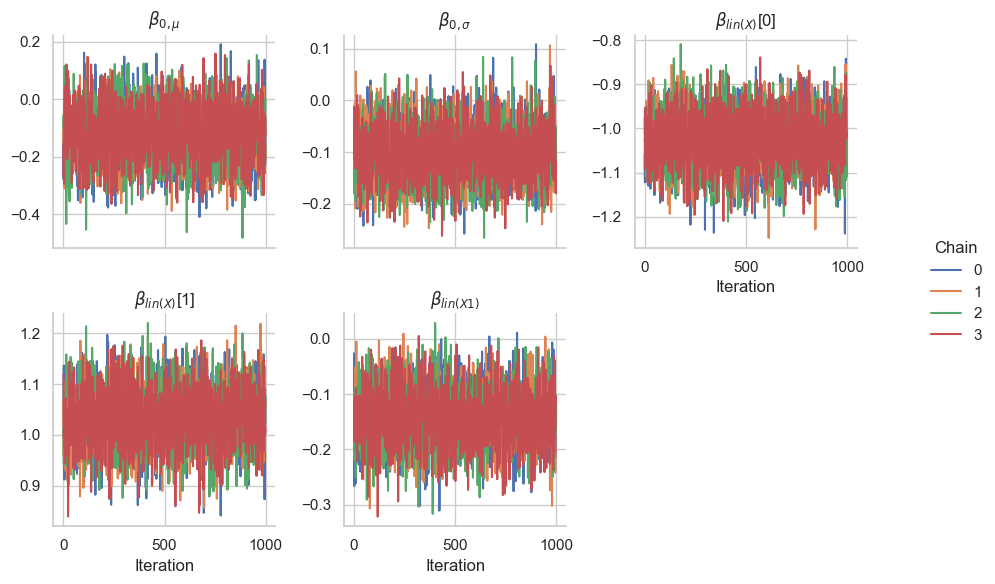
<seaborn.axisgrid.FacetGrid at 0x13dd2f610>

Predictions

samples = results.get_posterior_samples()

Predict variables at new x values

x_grid = jnp.linspace(x.min(), x.max(), 300)
predictions = model.predict(
    samples=samples,
    predict=["lin(X)", "lin(X1)", "$\\mu$", "$\\sigma$"],
    newdata={"x": x_grid},
)

predictions_summary = gs.SamplesSummary(predictions).to_dataframe().reset_index()
predictions_summary["x"] = np.tile(x_grid, len(predictions))

predictions_summary.head()

	variable	var_fqn	var_index	sample_size	mean	var	sd	ess_bulk	ess_tail	mcse_mean	mcse_sd	rhat	q_0.05	q_0.5	q_0.95	hdi_low	hdi_high	x
0	$\mu$	$\mu$[0]	(0,)	4000	5.947023	0.059801	0.244543	3230.505662	3651.905009	0.004305	0.002774	0.999674	5.534438	5.949018	6.350981	5.569644	6.370417	-1.976702
1	$\mu$	$\mu$[1]	(1,)	4000	5.879270	0.058344	0.241546	3239.614025	3651.586267	0.004247	0.002739	0.999643	5.471073	5.881016	6.278395	5.511409	6.302707	-1.963415
2	$\mu$	$\mu$[2]	(2,)	4000	5.811897	0.056917	0.238573	3245.814362	3687.244032	0.004190	0.002705	0.999632	5.408678	5.813008	6.206538	5.448952	6.231711	-1.950128
3	$\mu$	$\mu$[3]	(3,)	4000	5.744873	0.055519	0.235625	3252.757797	3687.244032	0.004133	0.002671	0.999623	5.346520	5.745001	6.134404	5.382929	6.156501	-1.936841
4	$\mu$	$\mu$[4]	(4,)	4000	5.678220	0.054150	0.232702	3261.208882	3651.458166	0.004076	0.002637	0.999619	5.284647	5.678637	6.062679	5.323129	6.088024	-1.923554

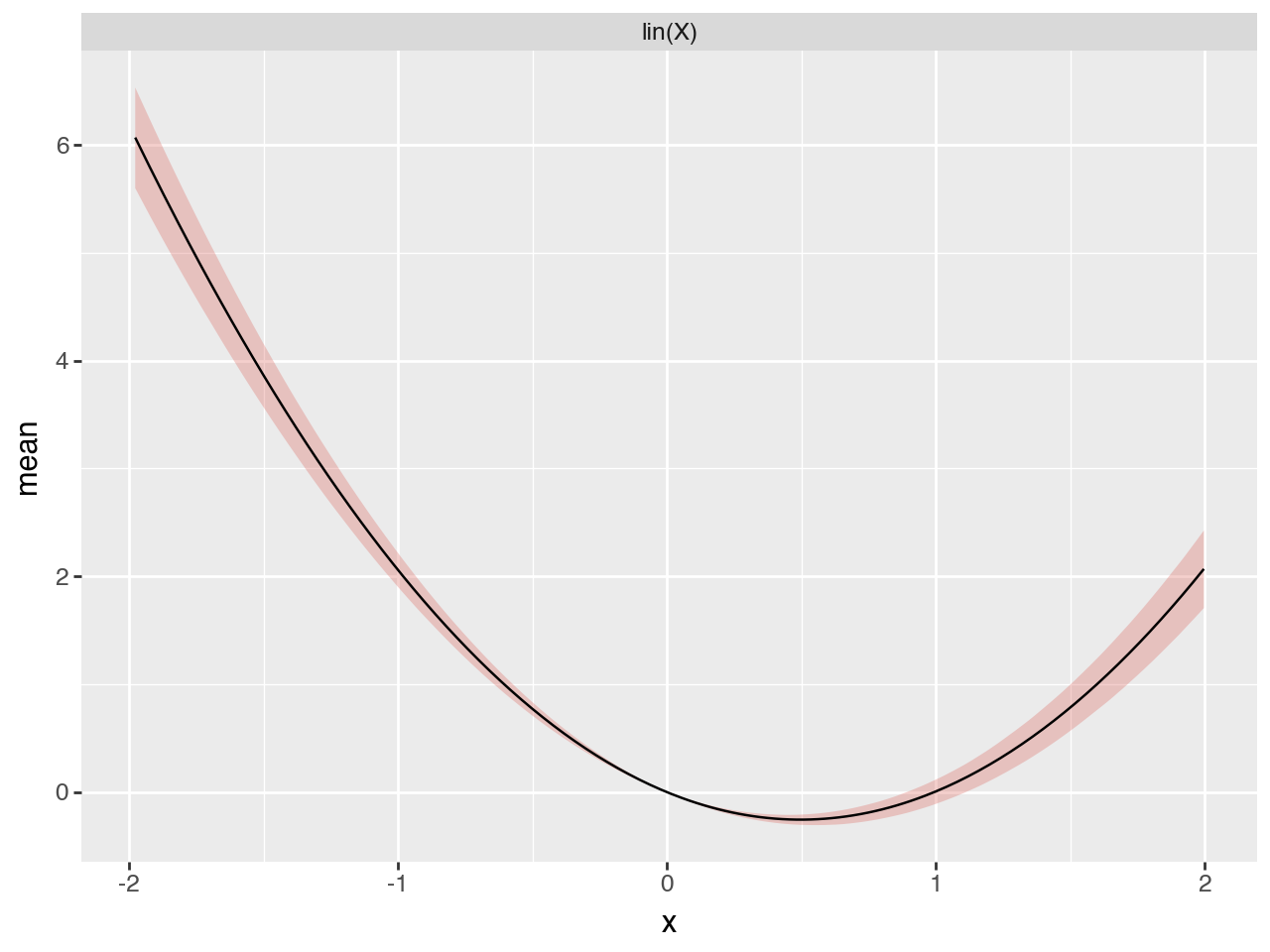
Plot fitted functions

select = predictions_summary["variable"].isin(["lin(X)", "lin(X2)"])
(
    p9.ggplot(predictions_summary[select])
    + p9.geom_ribbon(
        p9.aes("x", ymin="q_0.05", ymax="q_0.95", fill="variable"), alpha=0.3
    )
    + p9.geom_line(p9.aes("x", "mean"))
    + p9.facet_wrap("~variable", scales="free_y", ncol=1)
    + p9.guides(fill="none")
)

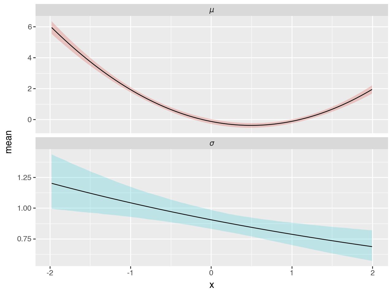
Plot parameters as functions of covariate

select = predictions_summary["variable"].isin(["$\\mu$", "$\\sigma$"])
(
    p9.ggplot(predictions_summary[select])
    + p9.geom_ribbon(
        p9.aes("x", ymin="q_0.05", ymax="q_0.95", fill="variable"), alpha=0.3
    )
    + p9.geom_line(p9.aes("x", "mean"))
    + p9.facet_wrap("~variable", scales="free_y", ncol=1)
    + p9.guides(fill="none")
)

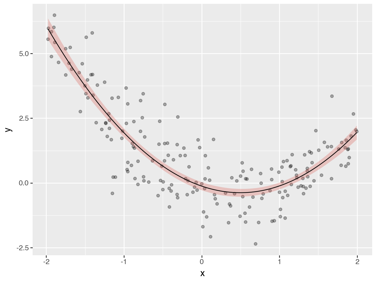
Plot mean function with data

select = predictions_summary["variable"].isin(["$\\mu$"])
(
    p9.ggplot(predictions_summary[select])
    + p9.geom_point(p9.aes("x", "y"), data=df, alpha=0.3)
    + p9.geom_ribbon(
        p9.aes("x", ymin="q_0.05", ymax="q_0.95", fill="variable"), alpha=0.3
    )
    + p9.geom_line(p9.aes("x", "mean"))
    + p9.guides(fill="none")
)

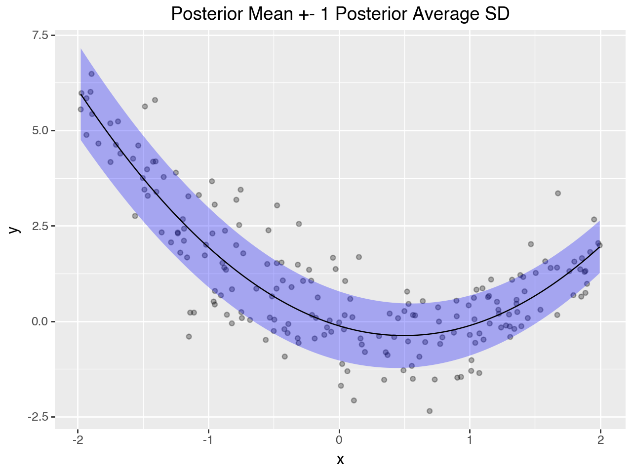
Plot average posterior predictive distribution

select = predictions_summary["variable"].isin(["$\\mu$", "$\\sigma$"])
mu_sigma_df = (
    predictions_summary[select][["variable", "mean", "x"]]
    .pivot(index="x", columns=["variable"], values="mean")
    .reset_index()
)

mu_sigma_df["low"] = mu_sigma_df["$\\mu$"] - mu_sigma_df["$\\sigma$"]
mu_sigma_df["high"] = mu_sigma_df["$\\mu$"] + mu_sigma_df["$\\sigma$"]
mu_sigma_df

variable	x	$\mu$	$\sigma$	low	high
0	-1.976702	5.947023	1.201194	4.745830	7.148217
1	-1.963415	5.879270	1.198869	4.680401	7.078139
2	-1.950128	5.811897	1.196550	4.615346	7.008447
3	-1.936841	5.744873	1.194239	4.550634	6.939112
4	-1.923554	5.678220	1.191927	4.486293	6.870147
...	...	...	...	...	...
295	1.942956	1.786320	0.691626	1.094695	2.477946
296	1.956243	1.826223	0.690378	1.135845	2.516601
297	1.969530	1.866492	0.689135	1.177358	2.555627
298	1.982817	1.907126	0.687889	1.219238	2.595015
299	1.996104	1.948120	0.686650	1.261469	2.634770

300 rows × 5 columns

(
    p9.ggplot()
    + p9.geom_point(p9.aes("x", "y"), data=df, alpha=0.3)
    + p9.geom_ribbon(
        p9.aes("x", ymin="low", ymax="high"),
        alpha=0.3,
        fill="blue",
        data=mu_sigma_df,
    )
    + p9.geom_line(p9.aes("x", "$\\mu$"), data=mu_sigma_df)
    + p9.labs(title="Posterior Mean +- 1 Posterior Average SD")
    + p9.guides(fill="none")
)

Posterior Predictive Checks

Draw posterior predictive samples

ppsamples = model.sample(shape=(3,), seed=jax.random.key(1), posterior_samples=samples)

ppsamples["y"].shape

(3, 4, 1000, 200)

# can be reshaped to concatenate the first two axes
_ = ppsamples["y"].reshape(-1, *ppsamples["y"].shape[2:])

Summarize posterior predictive samples

ppsamples = model.sample(
    shape=(),  # just draw 1 value for each posterior sample
    seed=jax.random.key(1),
    posterior_samples=samples,
)

# summarise ppsamples
ppsamples_summary = gs.SamplesSummary(ppsamples).to_dataframe().reset_index()

# add covariate to df
ppsamples_summary["x"] = df["x"].to_numpy()

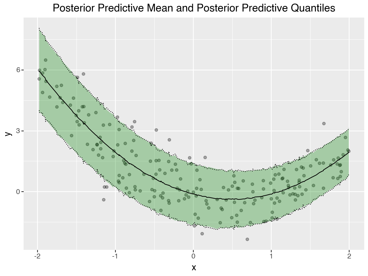
Plot posterior predictive summary

(
    p9.ggplot(ppsamples_summary)
    + p9.geom_point(p9.aes("x", "y"), data=df, alpha=0.3)
    + p9.geom_ribbon(
        p9.aes("x", ymin="q_0.05", ymax="q_0.95"),
        alpha=0.3,
        fill="green",
    )
    + p9.geom_line(p9.aes("x", "hdi_low"), linetype="dotted")
    + p9.geom_line(p9.aes("x", "hdi_high"), linetype="dotted")
    + p9.geom_line(p9.aes("x", "mean"))
    + p9.labs(title="Posterior Predictive Mean and Posterior Predictive Quantiles")
    + p9.guides(fill="none")
)

Plot posterior predictive samples

ppsamples_reshaped = ppsamples["y"].reshape(-1, *ppsamples["y"].shape[2:])
ppsamples_df = pd.DataFrame(ppsamples_reshaped.T)
ppsamples_df["x"] = df["x"].to_numpy()
ppsamples_df = ppsamples_df.melt(id_vars=["x"], value_name="y", var_name="sample")
ppsamples_df[ppsamples_df["sample"].isin(range(5))]


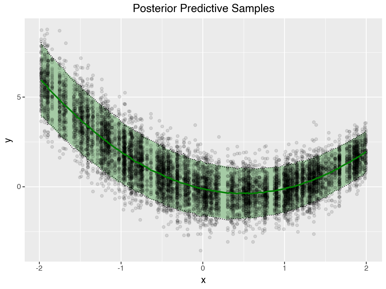
nsamples = 50


(
    p9.ggplot(ppsamples_df[ppsamples_df["sample"].isin(range(nsamples))])
    + p9.labs(title="Posterior Predictive Samples")
    + p9.geom_ribbon(
        p9.aes("x", ymin="q_0.05", ymax="q_0.95"),
        alpha=0.3,
        fill="green",
        data=ppsamples_summary,
    )
    + p9.geom_point(p9.aes("x", "y"), alpha=0.1)
    + p9.geom_line(p9.aes("x", "hdi_low"), linetype="dotted", data=ppsamples_summary)
    + p9.geom_line(p9.aes("x", "hdi_high"), linetype="dotted", data=ppsamples_summary)
    + p9.geom_line(p9.aes("x", "mean"), color="green", size=1, data=ppsamples_summary)
)