TX: Tensor Product Interaction

Setup and Imports

import jax.numpy as jnp
import liesel.goose as gs
import liesel.model as lsl
import matplotlib.pyplot as plt
import numpy as np
import plotnine as p9
import tensorflow_probability.substrates.jax.distributions as tfd

import liesel_gam as gam

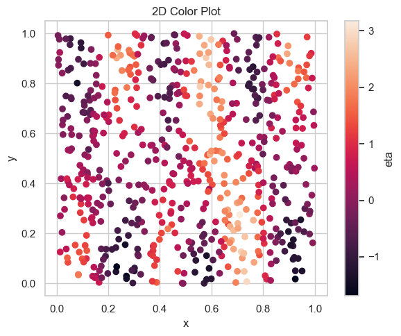
df = gam.demo_data_ta(n=600, noise_sd=0.25, seed=42)
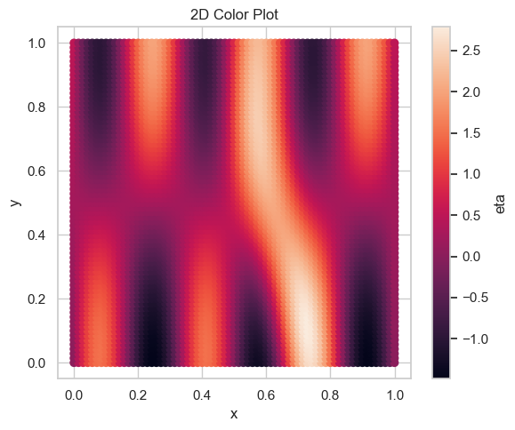
df_grid = gam.demo_data_ta(n=5000, grid=True)

plt.figure(figsize=(6, 5))
plt.scatter(df["x"], df["y"], c=df["z"])
plt.xlabel("x")
plt.ylabel("y")
plt.title("2D Color Plot")
plt.colorbar(label="eta")
plt.tight_layout()
plt.show()

plt.figure(figsize=(6, 5))
plt.scatter(df_grid["x"], df_grid["y"], c=df_grid["eta"])
plt.xlabel("x")
plt.ylabel("y")
plt.title("2D Color Plot")
plt.colorbar(label="eta")
plt.tight_layout()
plt.show()

Model Definition

Setup response model

loc = gam.AdditivePredictor("$\\mu$")
scale = gam.AdditivePredictor("$\\sigma$", inv_link=jnp.exp)


z = lsl.Var.new_obs(
    value=df.z.to_numpy(),
    distribution=lsl.Dist(tfd.Normal, loc=loc, scale=scale),
    name="z",
)

import tensorflow_probability.substrates.jax.bijectors as tfb


def scale_fn():
    prior = lsl.Dist(
        tfd.HalfNormal,
        scale=jnp.array(20.0),
    )

    scale = lsl.Var.new_param(
        jnp.array(0.1),
        distribution=prior,
        name="{x}",  # {x} is a placeholder for the automatically generated name
    )

    scale.transform(
        tfb.Softplus(),
        inference=gs.MCMCSpec(gs.IWLSKernel.untuned),
        name="h({x})",  # {x} is a placeholder for the automatically generated name
    )
    return scale


tb = gam.TermBuilder.from_df(df, default_scale_fn=scale_fn)

loc += tb.ps("x", k=15)
loc += tb.ps("y", k=15)


psx = tb.ps("x", k=12)
psy = tb.ps("y", k=12)

loc += tb.tx(psx, psy)

Build and plot model

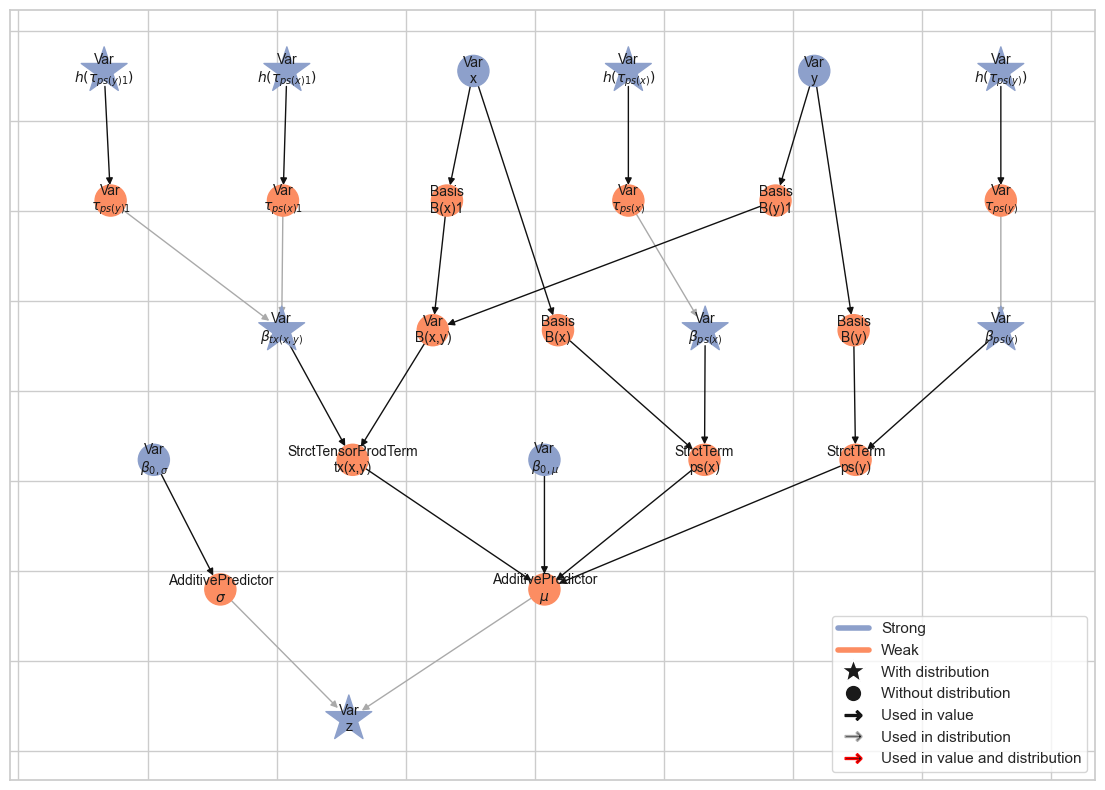
model = lsl.Model([z])
model.plot_vars()

liesel.model.model - INFO - Converted dtype of Value(name="z_value").value

Run MCMC

eb = gs.LieselMCMC(model).get_engine_builder(seed=1, num_chains=4)

eb.add_burnin(9000)
eb.add_posterior(10_000, thinning=10)
engine = eb.build()
engine.sample_all_epochs()
results = engine.get_results()

liesel.goose.builder - WARNING - No jitter functions provided for position keys '$\\beta_{0,\\sigma}$', '$\\beta_{0,\\mu}$', '$\\beta_{tx(x,y)}$', '$h(\\tau_{ps(y)1})$', '$h(\\tau_{ps(x)1})$', '$\\beta_{ps(y)}$', '$h(\\tau_{ps(y)})$', '$\\beta_{ps(x)}$', '$h(\\tau_{ps(x)})$'. The initial values for these keys won't be jittered
liesel.goose.engine - INFO - Initializing kernels...
liesel.goose.engine - INFO - Done
liesel.goose.engine - INFO - Starting epoch: BURNIN, 9000 transitions, 1000 jitted together
100%|██████████████████████████████████████████| 9/9 [00:15<00:00,  1.78s/chunk]
liesel.goose.engine - WARNING - Errors per chain for kernel_04: 35, 334, 33, 31 / 9000 transitions
liesel.goose.engine - WARNING - Errors per chain for kernel_06: 1, 2, 0, 0 / 9000 transitions
liesel.goose.engine - WARNING - Errors per chain for kernel_08: 0, 0, 1, 1 / 9000 transitions
liesel.goose.engine - INFO - Finished epoch
liesel.goose.engine - INFO - Finished warmup
liesel.goose.engine - INFO - Starting epoch: POSTERIOR, 10000 transitions, 1000 jitted together
100%|████████████████████████████████████████| 10/10 [00:17<00:00,  1.73s/chunk]
liesel.goose.engine - WARNING - Errors per chain for kernel_04: 47, 31, 41, 39 / 10000 transitions
liesel.goose.engine - INFO - Finished epoch

MCMC summary

summary = gs.Summary(results)

diagnostics = (
    summary.to_dataframe()
    .reset_index()
    .loc[:, ["variable", "rhat", "ess_bulk", "ess_tail"]]
    .groupby("variable", as_index=False)
    .agg(
        ess_bulk_min=("ess_bulk", "min"),
        ess_bulk_median=("ess_bulk", "median"),
        ess_tail_min=("ess_tail", "min"),
        ess_tail_median=("ess_tail", "median"),
        rhat_max=("rhat", "max"),
        rhat_median=("rhat", "median"),
    )
)
diagnostics

	variable	ess_bulk_min	ess_bulk_median	ess_tail_min	ess_tail_median	rhat_max	rhat_median
0	$\beta_{0,\mu}$	3474.404855	3474.404855	3971.892421	3971.892421	1.000077	1.000077
1	$\beta_{0,\sigma}$	1752.446589	1752.446589	3211.706173	3211.706173	1.001632	1.001632
2	$\beta_{ps(x)}$	2961.800854	3349.946500	3187.134612	3568.053819	1.000867	1.000310
3	$\beta_{ps(y)}$	971.321747	2578.406339	1056.506165	1811.451052	1.009294	1.005722
4	$\beta_{tx(x,y)}$	300.804955	1468.151829	800.148723	1688.467815	1.026784	1.003717
5	$h(\tau_{ps(x)1})$	2971.149153	2971.149153	2610.390712	2610.390712	1.000495	1.000495
6	$h(\tau_{ps(x)})$	2878.984591	2878.984591	3330.797473	3330.797473	0.999342	0.999342
7	$h(\tau_{ps(y)1})$	150.138651	150.138651	287.366766	287.366766	1.044090	1.044090
8	$h(\tau_{ps(y)})$	404.461391	404.461391	732.995655	732.995655	1.021952	1.021952

summary.error_df()

				count	sample_size	sample_size_total	relative
kernel	error_code	error_msg	phase
kernel_04	90	nan acceptance prob	warmup	433	36000	36000	0.012028
			posterior	158	4000	40000	0.00395
kernel_06	90	nan acceptance prob	warmup	3	36000	36000	0.000083
			posterior	0	4000	40000	0.0
kernel_08	90	nan acceptance prob	warmup	2	36000	36000	0.000056
			posterior	0	4000	40000	0.0

gs.plot_trace(results, [n for n in model.parameters if "tau" in n])

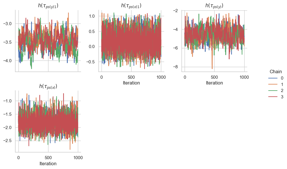
<seaborn.axisgrid.FacetGrid at 0x14deb1310>

samples = results.get_posterior_samples()

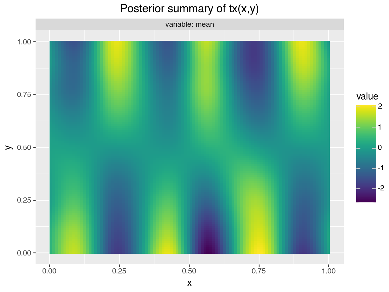
gam.plot_2d_smooth(model.vars["tx(x,y)"], samples, ngrid=100)

gs.plot_trace(
    model.predict(samples, predict=[s.name for s in model.vars["tx(x,y)"].scales])
)

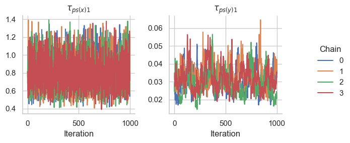
<seaborn.axisgrid.FacetGrid at 0x14de9fd90>

MCMC trace plots

Predictions

samples = results.get_posterior_samples()

Predict variables at new x values

predictions = model.predict(
    samples=samples,
    predict=["$\\mu$"],
    newdata={"x": df_grid.x.to_numpy(), "y": df_grid.y.to_numpy()},
)

predictions_summary = (
    gs.SamplesSummary(predictions, which=["mean", "quantiles"])
    .to_dataframe()
    .reset_index()
)

predictions_summary["x"] = np.tile(df_grid.x.to_numpy(), len(predictions))
predictions_summary["y"] = np.tile(df_grid.y.to_numpy(), len(predictions))

predictions_summary.head()

	variable	var_fqn	var_index	sample_size	mean	q_0.05	q_0.5	q_0.95	x	y
0	$\mu$	$\mu$[0]	(0,)	4000	0.221714	-0.796235	0.216299	1.231756	0.000000	0.0
1	$\mu$	$\mu$[1]	(1,)	4000	0.587376	-0.198893	0.580743	1.381314	0.014286	0.0
2	$\mu$	$\mu$[2]	(2,)	4000	0.929080	0.297584	0.928636	1.550423	0.028571	0.0
3	$\mu$	$\mu$[3]	(3,)	4000	1.229069	0.700319	1.233325	1.742260	0.042857	0.0
4	$\mu$	$\mu$[4]	(4,)	4000	1.470111	1.023793	1.480602	1.905741	0.057143	0.0

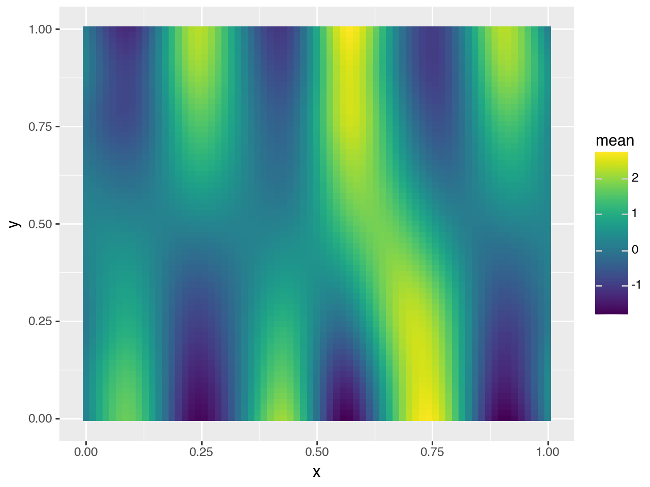
Plot fitted functions

select = predictions_summary["variable"].isin(["$\\mu$"])
(p9.ggplot(predictions_summary[select]) + p9.geom_tile(p9.aes("x", "y", fill="mean")))

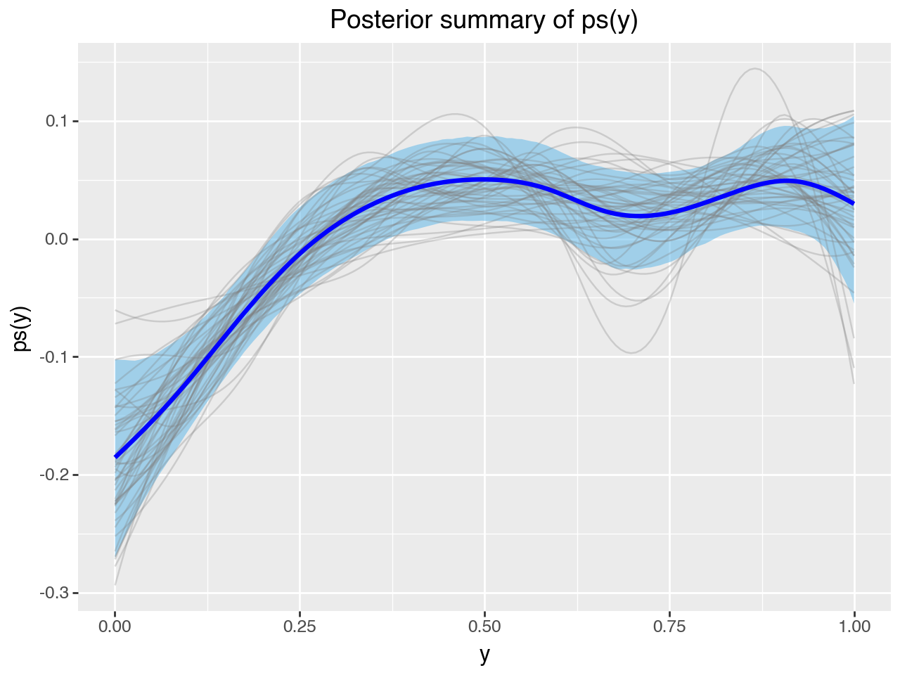
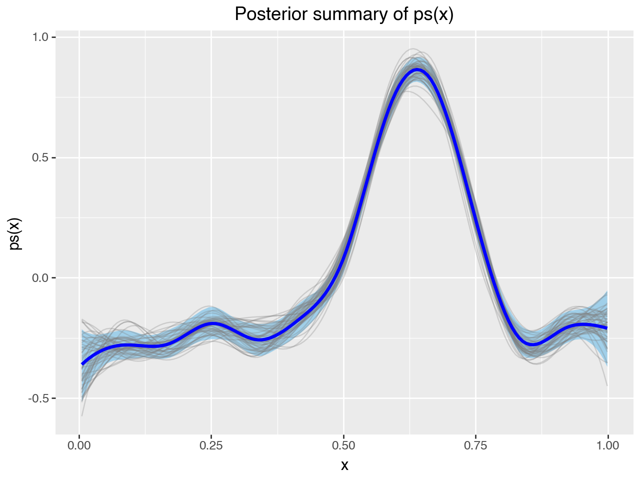
gam.plot_1d_smooth(model.vars["ps(x)"], samples)

gam.plot_1d_smooth(model.vars["ps(y)"], samples)