TX: Tensor Product Interaction with pre-optimization

Contents

TX: Tensor Product Interaction with pre-optimization#

This notebook shows an exmaple of how to use liesel_gam.consolidate_bases to turn weak basis matrix variables into strong ones - this can be necessary to avoid problems with callbacks to R, especially when trying to optimize for good starting values using liesel.goose.optim_flat.

Setup and Imports#

import jax.numpy as jnp
import liesel.goose as gs
import liesel.model as lsl
import matplotlib.pyplot as plt
import numpy as np
import plotnine as p9
import tensorflow_probability.substrates.jax.distributions as tfd

import liesel_gam as gam
from liesel_gam.consolidate_bases import consolidate_bases, evaluate_bases

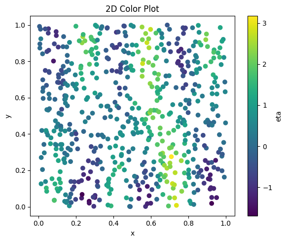
df = gam.demo_data_ta(n=600, noise_sd=0.25, seed=42)
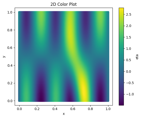
df_grid = gam.demo_data_ta(n=5000, grid=True)

plt.figure(figsize=(6, 5))
plt.scatter(df["x"], df["y"], c=df["z"])
plt.xlabel("x")
plt.ylabel("y")
plt.title("2D Color Plot")
plt.colorbar(label="eta")
plt.tight_layout()
plt.show()

../../_images/3cc856778a249c72b0e47f4780da6b1626ec49b914ddb26c260b99ba18462f18.png

plt.figure(figsize=(6, 5))
plt.scatter(df_grid["x"], df_grid["y"], c=df_grid["eta"])
plt.xlabel("x")
plt.ylabel("y")
plt.title("2D Color Plot")
plt.colorbar(label="eta")
plt.tight_layout()
plt.show()

../../_images/442782da995afa1e1b5a6cfe829a735b6a6a81abae661021bce762ead606523e.png

Model Definition#

Setup response model#

loc = gam.AdditivePredictor("$\\mu$")
scale = gam.AdditivePredictor("$\\sigma$", inv_link=jnp.exp)


z = lsl.Var.new_obs(
    value=df.z.to_numpy(),
    distribution=lsl.Dist(tfd.Normal, loc=loc, scale=scale),
    name="z",
)

import tensorflow_probability.substrates.jax.bijectors as tfb


def scale_fn():
    prior = lsl.Dist(
        tfd.HalfNormal,
        scale=jnp.array(20.0),
    )

    scale = lsl.Var.new_param(
        jnp.array(0.1),
        distribution=prior,
        name="{x}",  # {x} is a placeholder for the automatically generated name
    )

    scale.transform(
        tfb.Softplus(),
        inference=gs.MCMCSpec(gs.IWLSKernel.untuned),
        name="h({x})",  # {x} is a placeholder for the automatically generated name
    )
    return scale


tb = gam.TermBuilder.from_df(df, default_scale_fn=scale_fn)

loc += (
    tb.ps("x", k=20),
    tb.ps("y", k=20),
    tb.tx(
        tb.ps("x", k=10),
        tb.ps("y", k=10),
    ),
)

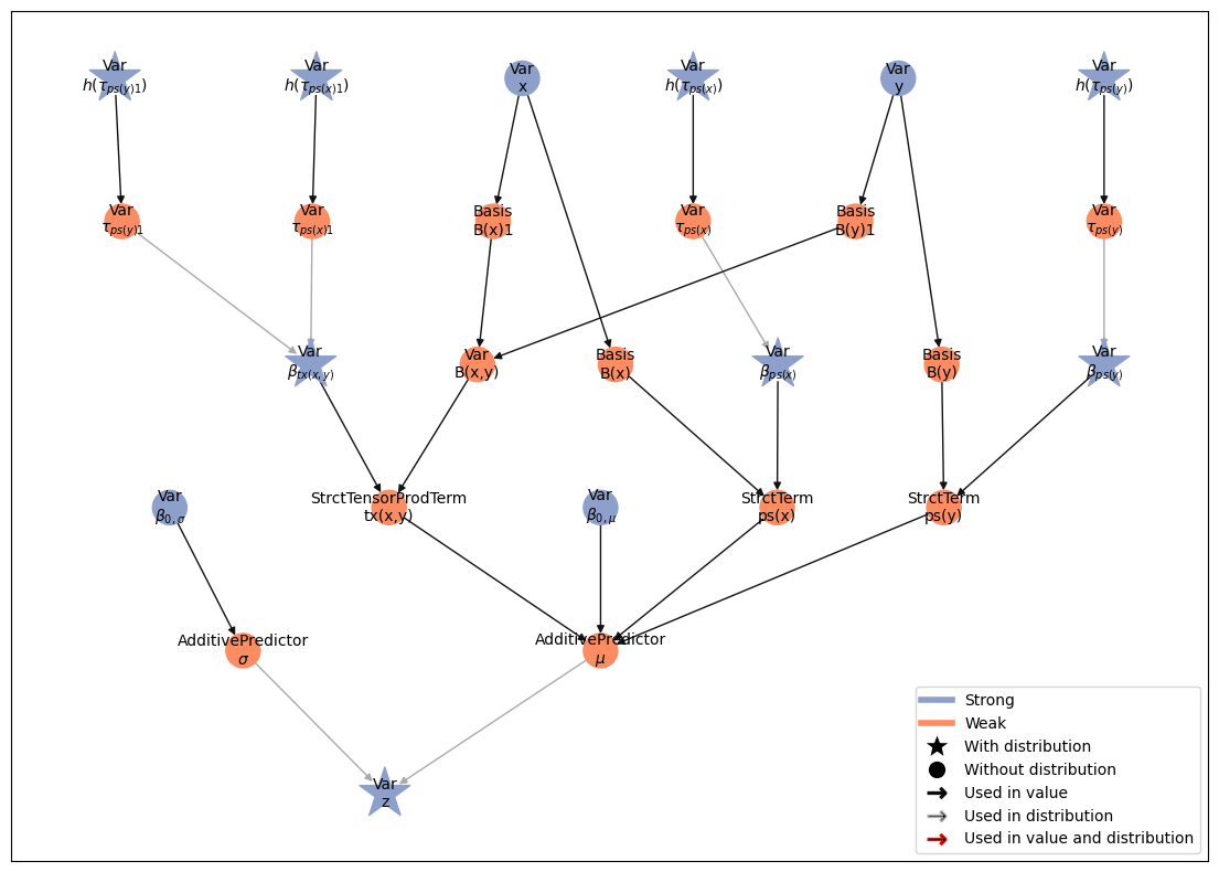
Build and plot model#

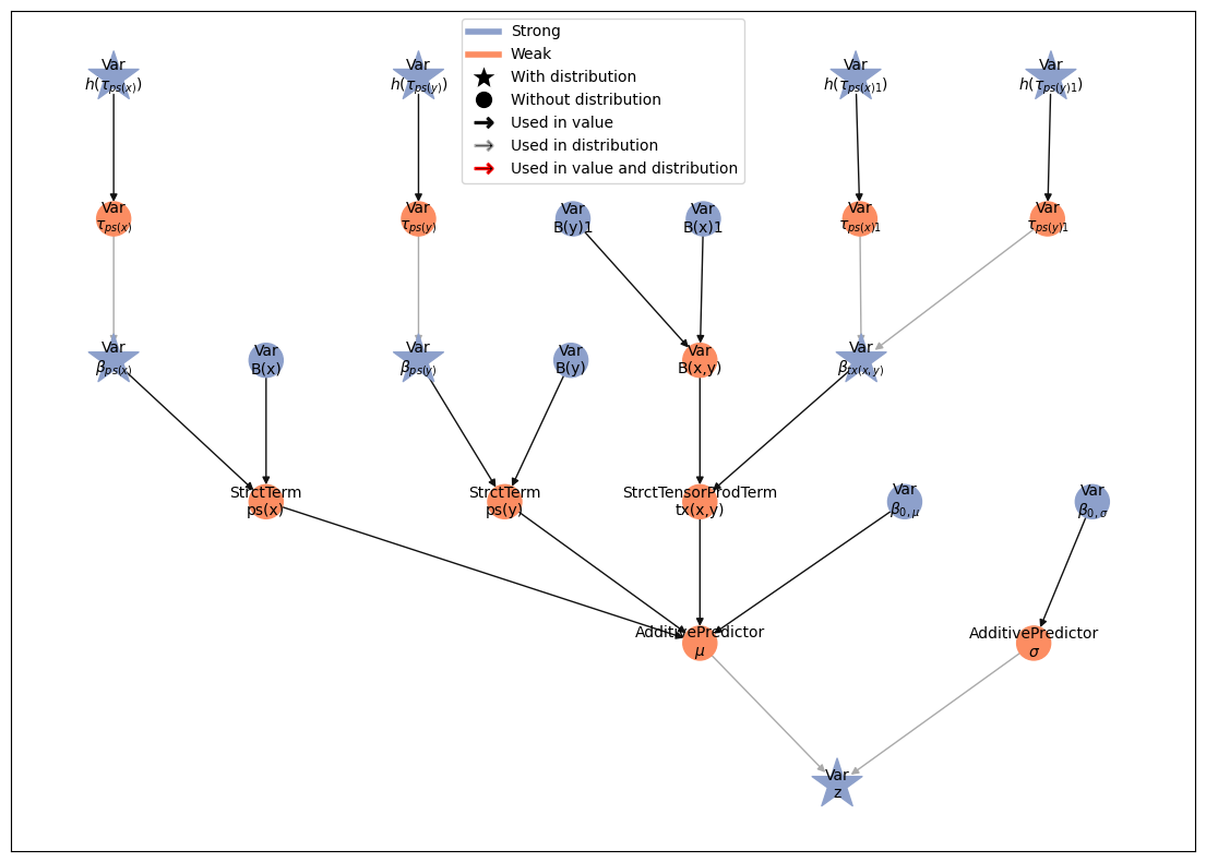
model = lsl.Model([z])
model.plot_vars()

liesel.model.model - INFO - Converted dtype of Value(name="z_value").value

../../_images/4672373351a864b8e8ca56e8c88b028ec4a26b85562481569261bf88addaa35f.png

model, bases_model = consolidate_bases(model)

bases_model.plot_vars()

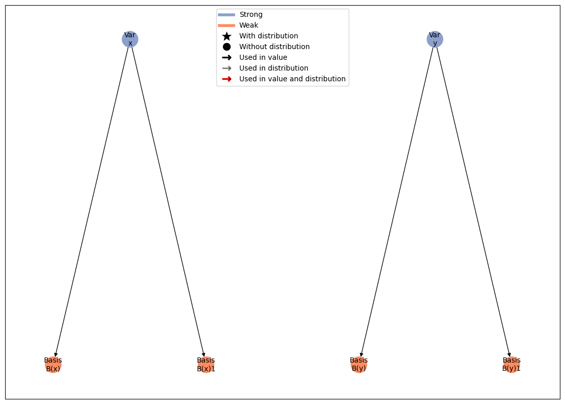
../../_images/73f99695b95605e70d7026466051336bf96cad0d47dbc708e0036edcb13179f9.png

model.plot_vars()

../../_images/6a18aad1b052e30a0b3cf5810b97ba12b10f081bb77cb08b82c1ecf5a7a00c1c.png

import optax

params = [p.name for p in model.parameters.values() if not p.name.startswith("$\\tau")]

# this is the optimization
# I am being lazy here: Usually, convergence should be assessed.
opt = gs.optim_flat(
    model,
    params,
    optimizer=optax.adam(learning_rate=1e-3),
    progress_bar=False,
)

model.state = model.update_state(opt.position)

Run MCMC#

eb = gs.LieselMCMC(model).get_engine_builder(seed=1, num_chains=4)

eb.add_adaptation(2000)
eb.add_posterior(5000, thinning=5)

engine = eb.build()
engine.sample_all_epochs()
results = engine.get_results()

liesel.goose.builder - WARNING - No jitter functions provided for position keys '$h(\\tau_{ps(x)})$', '$\\beta_{ps(x)}$', '$h(\\tau_{ps(y)})$', '$\\beta_{ps(y)}$', '$h(\\tau_{ps(x)1})$', '$h(\\tau_{ps(y)1})$', '$\\beta_{tx(x,y)}$', '$\\beta_{0,\\mu}$', '$\\beta_{0,\\sigma}$'. The initial values for these keys won't be jittered
liesel.goose.engine - INFO - Initializing kernels...
liesel.goose.engine - INFO - Done
liesel.goose.engine - INFO - Starting epoch: FAST_ADAPTATION, 200 transitions, 25 jitted together
100%|██████████████████████████████████████████| 8/8 [00:13<00:00,  1.70s/chunk]
liesel.goose.engine - WARNING - Errors per chain for kernel_04: 4, 1, 3, 3 / 200 transitions
liesel.goose.engine - INFO - Finished epoch
liesel.goose.engine - INFO - Starting epoch: SLOW_ADAPTATION, 25 transitions, 25 jitted together
100%|█████████████████████████████████████████| 1/1 [00:00<00:00, 819.68chunk/s]
liesel.goose.engine - WARNING - Errors per chain for kernel_04: 0, 1, 0, 1 / 25 transitions
liesel.goose.engine - INFO - Finished epoch
liesel.goose.engine - INFO - Starting epoch: SLOW_ADAPTATION, 50 transitions, 25 jitted together
100%|████████████████████████████████████████| 2/2 [00:00<00:00, 1110.49chunk/s]
liesel.goose.engine - WARNING - Errors per chain for kernel_04: 0, 0, 3, 2 / 50 transitions
liesel.goose.engine - INFO - Finished epoch
liesel.goose.engine - INFO - Starting epoch: SLOW_ADAPTATION, 100 transitions, 25 jitted together
100%|████████████████████████████████████████| 4/4 [00:00<00:00, 1378.80chunk/s]
liesel.goose.engine - WARNING - Errors per chain for kernel_04: 0, 1, 2, 0 / 100 transitions
liesel.goose.engine - INFO - Finished epoch
liesel.goose.engine - INFO - Starting epoch: SLOW_ADAPTATION, 200 transitions, 25 jitted together
100%|█████████████████████████████████████████| 8/8 [00:00<00:00, 214.18chunk/s]
liesel.goose.engine - WARNING - Errors per chain for kernel_04: 7, 5, 4, 1 / 200 transitions
liesel.goose.engine - INFO - Finished epoch
liesel.goose.engine - INFO - Starting epoch: SLOW_ADAPTATION, 1025 transitions, 25 jitted together
100%|████████████████████████████████████████| 41/41 [00:01<00:00, 36.39chunk/s]
liesel.goose.engine - WARNING - Errors per chain for kernel_04: 14, 18, 24, 14 / 1025 transitions
liesel.goose.engine - INFO - Finished epoch
liesel.goose.engine - INFO - Starting epoch: FAST_ADAPTATION, 400 transitions, 25 jitted together
100%|████████████████████████████████████████| 16/16 [00:00<00:00, 55.35chunk/s]
liesel.goose.engine - WARNING - Errors per chain for kernel_04: 4, 6, 12, 4 / 400 transitions
liesel.goose.engine - INFO - Finished epoch
liesel.goose.engine - INFO - Finished warmup
liesel.goose.engine - INFO - Starting epoch: POSTERIOR, 5000 transitions, 25 jitted together
100%|██████████████████████████████████████| 200/200 [00:06<00:00, 29.24chunk/s]
liesel.goose.engine - WARNING - Errors per chain for kernel_04: 97, 99, 95, 141 / 5000 transitions
liesel.goose.engine - INFO - Finished epoch

MCMC summary#

summary = gs.Summary(results)

diagnostics = (
    summary.to_dataframe()
    .reset_index()
    .loc[:, ["variable", "rhat", "ess_bulk", "ess_tail"]]
    .groupby("variable", as_index=False)
    .agg(
        ess_bulk_min=("ess_bulk", "min"),
        ess_bulk_median=("ess_bulk", "median"),
        ess_tail_min=("ess_tail", "min"),
        ess_tail_median=("ess_tail", "median"),
        rhat_max=("rhat", "max"),
        rhat_median=("rhat", "median"),
    )
)
diagnostics

	variable	ess_bulk_min	ess_bulk_median	ess_tail_min	ess_tail_median	rhat_max	rhat_median
0	$\beta_{0,\mu}$	3307.507975	3307.507975	3577.557442	3577.557442	1.002009	1.002009
1	$\beta_{0,\sigma}$	918.366039	918.366039	2255.471602	2255.471602	1.001283	1.001283
2	$\beta_{ps(x)}$	1712.997026	2584.969387	2731.346476	3141.713481	1.001389	1.000966
3	$\beta_{ps(y)}$	546.610660	2569.339449	718.818928	1253.673204	1.010668	1.008388
4	$\beta_{tx(x,y)}$	150.340189	1161.144110	422.045756	1315.808045	1.018642	1.003531
5	$h(\tau_{ps(x)1})$	1005.764434	1005.764434	412.597416	412.597416	1.005035	1.005035
6	$h(\tau_{ps(x)})$	1204.391135	1204.391135	2110.485263	2110.485263	1.000669	1.000669
7	$h(\tau_{ps(y)1})$	111.437076	111.437076	334.814216	334.814216	1.018971	1.018971
8	$h(\tau_{ps(y)})$	157.634193	157.634193	208.067725	208.067725	1.027667	1.027667

Predictions#

samples = results.get_posterior_samples()

newdata = {"x": df_grid.x.to_numpy(), "y": df_grid.y.to_numpy()}
newdata = evaluate_bases(newdata, bases_model)

Predict variables at new x values#

predictions = model.predict(
    samples=samples,
    predict=["tx(x,y)", "$\\mu$", "ps(x)", "ps(y)"],
    newdata=newdata,
)

predictions_summary = (
    gs.SamplesSummary(predictions, which=["mean", "quantiles"])
    .to_dataframe()
    .reset_index()
)

predictions_summary["x"] = np.tile(df_grid.x.to_numpy(), len(predictions))
predictions_summary["y"] = np.tile(df_grid.y.to_numpy(), len(predictions))

predictions_summary.head()

	variable	var_fqn	var_index	sample_size	mean	q_0.05	q_0.5	q_0.95	x	y
0	$\mu$	$\mu$[0]	(0,)	4000	-0.794277	-1.919930	-0.804964	0.356087	0.000000	0.0
1	$\mu$	$\mu$[1]	(1,)	4000	0.192279	-0.705666	0.190628	1.091368	0.014286	0.0
2	$\mu$	$\mu$[2]	(2,)	4000	0.934204	0.219105	0.930426	1.650856	0.028571	0.0
3	$\mu$	$\mu$[3]	(3,)	4000	1.442272	0.857040	1.448904	2.031990	0.042857	0.0
4	$\mu$	$\mu$[4]	(4,)	4000	1.740637	1.258972	1.745124	2.231986	0.057143	0.0

Plot fitted functions#

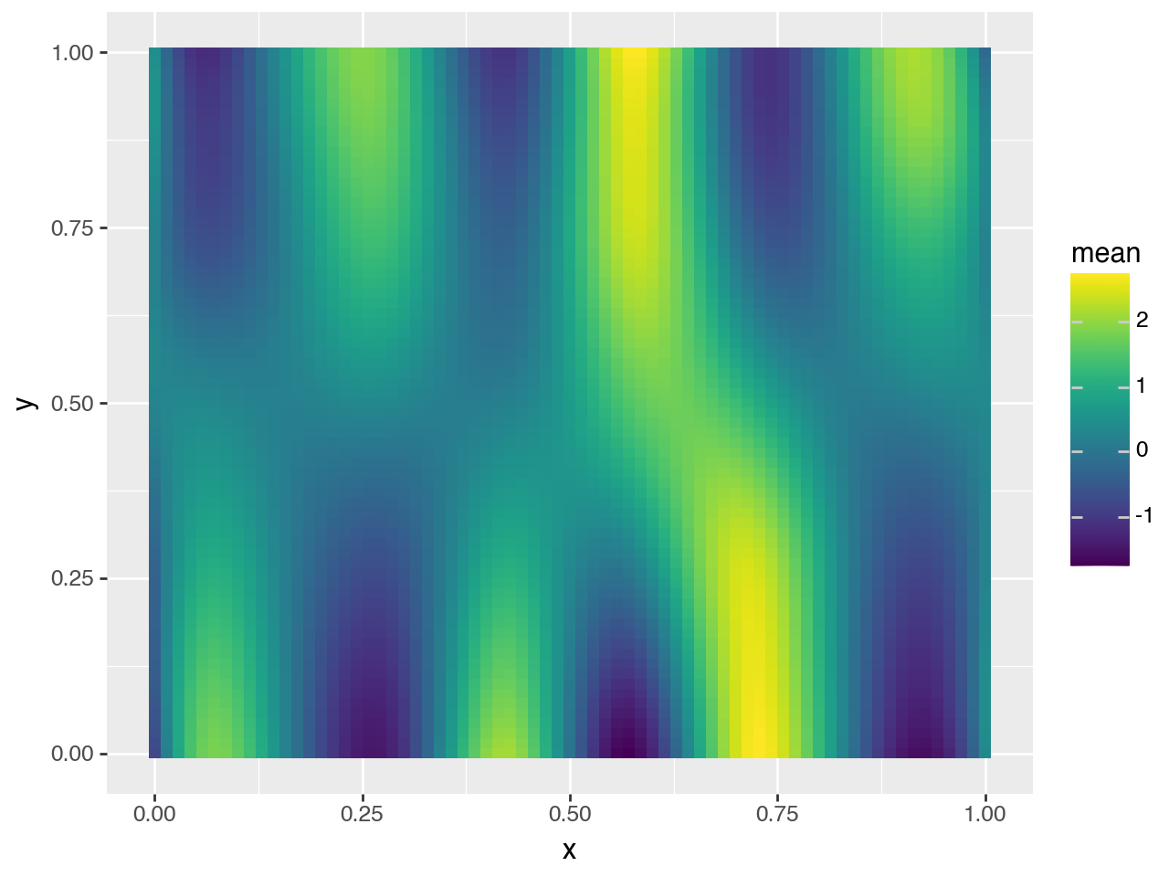
select = predictions_summary["variable"].isin(["tx(x,y)"])
(p9.ggplot(predictions_summary[select]) + p9.geom_tile(p9.aes("x", "y", fill="mean")))

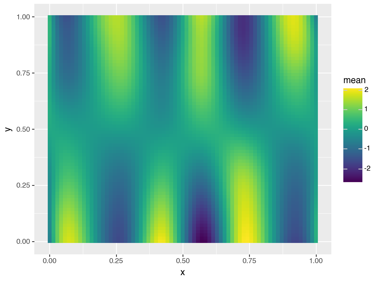
../../_images/b918b6c877a1d61da06b700b8e78b0e4c7f85e433241dcc0ad99858b05aec44d.png

select = predictions_summary["variable"].isin(["$\\mu$"])
(p9.ggplot(predictions_summary[select]) + p9.geom_tile(p9.aes("x", "y", fill="mean")))

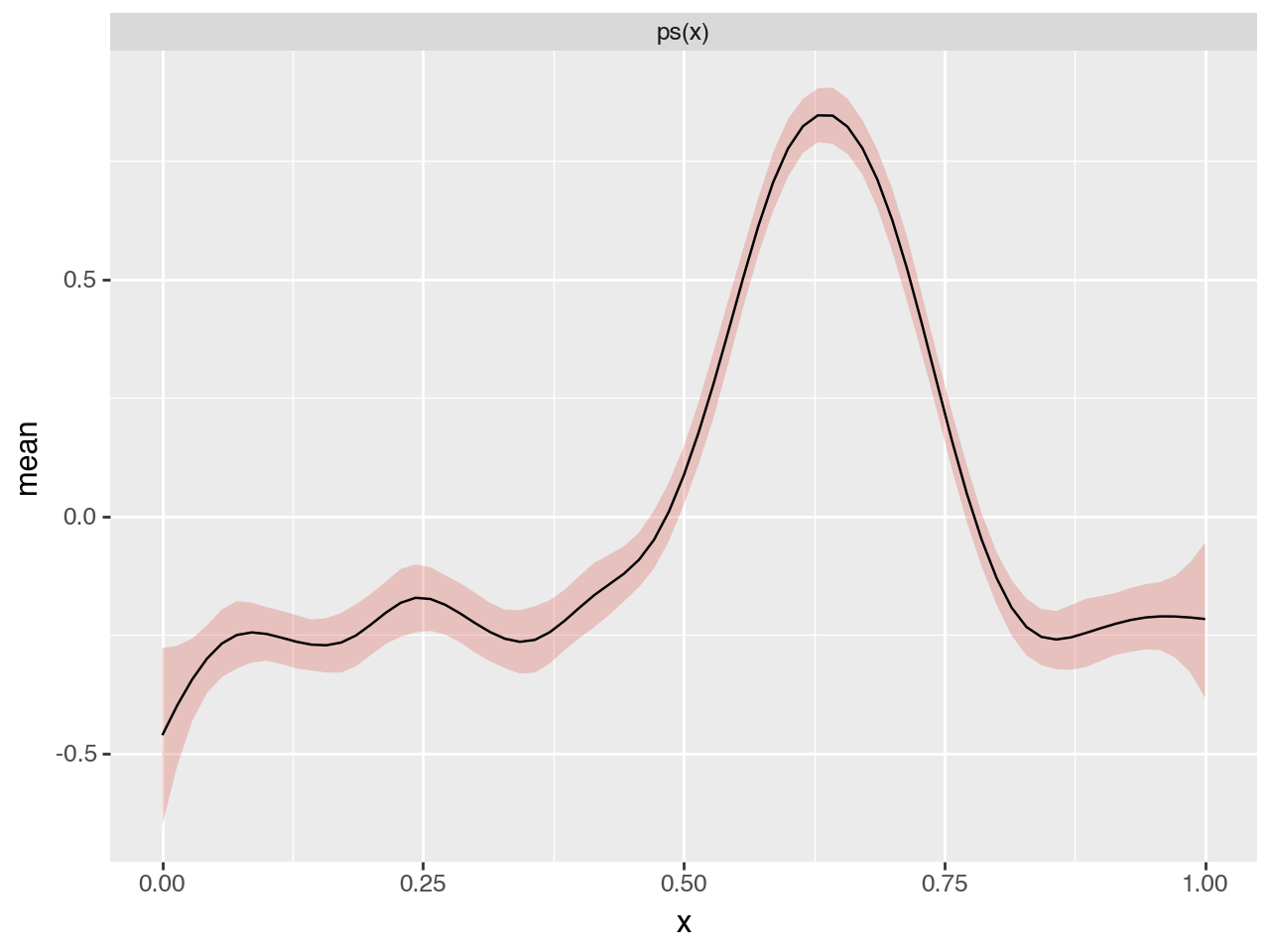
../../_images/af10d6935d106306eca0a4690cde6687a860a55d81b3fbba27dd10beb00f0c33.png

select = predictions_summary["variable"].isin(["ps(x)"])
(
    p9.ggplot(predictions_summary[select])
    + p9.geom_ribbon(
        p9.aes("x", ymin="q_0.05", ymax="q_0.95", fill="variable"), alpha=0.3
    )
    + p9.geom_line(p9.aes("x", "mean"))
    + p9.facet_wrap("~variable", scales="free_y", ncol=1)
    + p9.guides(fill="none")
)

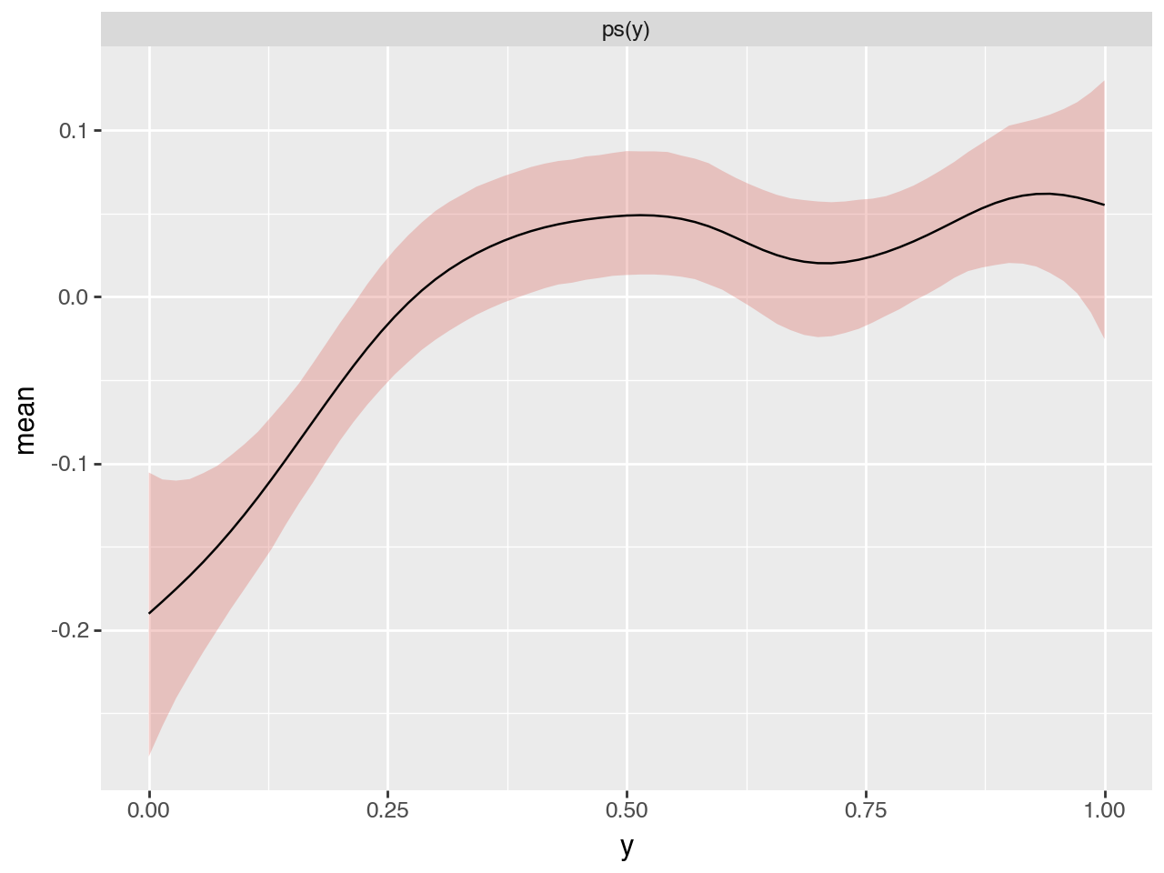
../../_images/d653679e4ae81ef5bfe02934940602019e0da6847266d5c83cf4dae5bd905f84.png

select = predictions_summary["variable"].isin(["ps(y)"])
(
    p9.ggplot(predictions_summary[select])
    + p9.geom_ribbon(
        p9.aes("y", ymin="q_0.05", ymax="q_0.95", fill="variable"), alpha=0.3
    )
    + p9.geom_line(p9.aes("y", "mean"))
    + p9.facet_wrap("~variable", scales="free_y", ncol=1)
    + p9.guides(fill="none")
)

../../_images/137c929c68827866b93e9824df25ec0d205c973bb56346aab5cf8181421a7736.png