PS: P-Spline

Setup and Imports

import jax.numpy as jnp
import liesel.goose as gs
import liesel.model as lsl
import numpy as np
import pandas as pd
import plotnine as p9
import tensorflow_probability.substrates.jax.distributions as tfd

import liesel_gam as gam

from scipy import stats

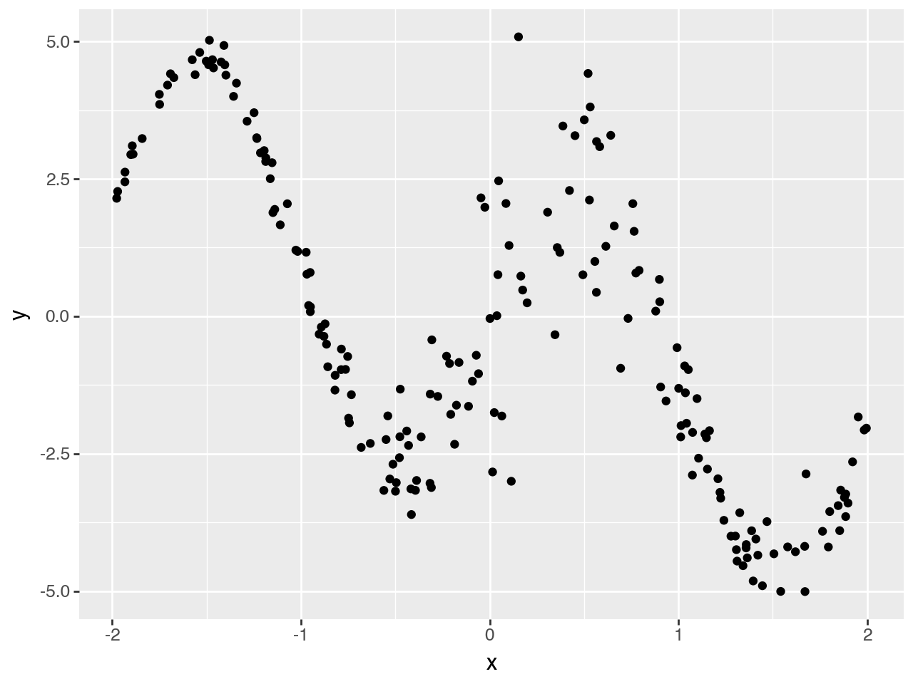
rng = np.random.default_rng(1)
x = rng.uniform(-2, 2, 200)

log_sigma = -1.0 + 0.3 * (
    0.5 * x + 15 * stats.norm.pdf(2 * (x - 0.2)) - stats.norm.pdf(x + 0.4)
)
mu = -x + np.pi * np.sin(np.pi * x)
y = mu + jnp.exp(log_sigma) * rng.normal(0.0, 1.0, 200)

df = pd.DataFrame({"y": y, "x": x})

(p9.ggplot(df) + p9.geom_point(p9.aes("x", "y")))

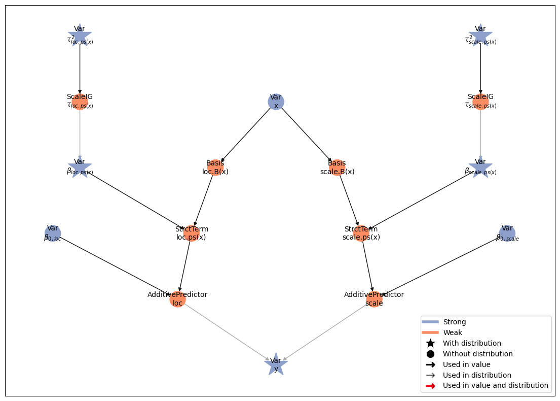
Model Definition

Setup response model

loc = gam.AdditivePredictor("loc")
scale = gam.AdditivePredictor("scale", inv_link=jnp.exp)


y = lsl.Var.new_obs(
    value=df.y.to_numpy(),
    distribution=lsl.Dist(tfd.Normal, loc=loc, scale=scale),
    name="y",
)


registry = gam.PandasRegistry(df)
tbl = gam.TermBuilder(registry, prefix_names_by="loc.")
tbs = gam.TermBuilder(registry, prefix_names_by="scale.")

loc += tbl.ps("x", k=20)
scale += tbs.ps("x", k=20)

Build and plot model

model = lsl.Model([y])
model.plot_vars()

Run MCMC

eb = gs.LieselMCMC(model).get_engine_builder(seed=1, num_chains=4)

eb.add_burnin(3000)
eb.add_posterior(10_000, thinning=10)

engine = eb.build()
engine.sample_all_epochs()
results = engine.get_results()

liesel.goose.builder - WARNING - No jitter functions provided for position keys '$\\beta_{0,scale}$', '$\\beta_{scale.ps(x)}$', '$\\tau_{scale.ps(x)}^2$', '$\\beta_{0,loc}$', '$\\beta_{loc.ps(x)}$', '$\\tau_{loc.ps(x)}^2$'. The initial values for these keys won't be jittered
liesel.goose.engine - INFO - Initializing kernels...
liesel.goose.engine - INFO - Done
liesel.goose.engine - INFO - Starting epoch: BURNIN, 3000 transitions, 1000 jitted together
100%|██████████████████████████████████████████| 3/3 [00:05<00:00,  1.82s/chunk]
liesel.goose.engine - INFO - Finished epoch
liesel.goose.engine - INFO - Finished warmup
liesel.goose.engine - INFO - Starting epoch: POSTERIOR, 10000 transitions, 1000 jitted together
100%|████████████████████████████████████████| 10/10 [00:03<00:00,  3.07chunk/s]
liesel.goose.engine - INFO - Finished epoch

MCMC summary

summary = gs.Summary(results)
summary

Parameter summary:

		kernel	mean	sd	q_0.05	q_0.5	q_0.95	sample_size	ess_bulk	ess_tail	rhat
parameter	index
$\beta_{0,loc}$	()	kernel_03	-0.319038	0.057453	-0.416217	-0.318389	-0.226010	4000	755.160850	1507.577246	1.006317
$\beta_{0,scale}$	()	kernel_00	-0.628547	0.053395	-0.716780	-0.629166	-0.538788	4000	3761.400457	3853.334601	0.999635
$\beta_{loc.ps(x)}$	(0,)	kernel_04	0.161261	0.337669	-0.384076	0.158211	0.713702	4000	3516.217015	3957.553226	0.999434
	(1,)	kernel_04	-0.138344	0.302521	-0.630288	-0.137469	0.333897	4000	3139.145645	4010.632015	1.000148
	(2,)	kernel_04	0.146713	0.308337	-0.345811	0.137165	0.652972	4000	3514.173945	3697.127246	0.999948
	(3,)	kernel_04	0.160964	0.288147	-0.300860	0.156749	0.643485	4000	3908.215895	3771.215333	1.000821
	(4,)	kernel_04	-0.263484	0.283364	-0.745345	-0.255425	0.192801	4000	3612.154260	3708.645519	1.000955
	(5,)	kernel_04	0.015893	0.268138	-0.417609	0.015399	0.460677	4000	3608.825471	3651.776257	1.000250
	(6,)	kernel_04	0.004710	0.250642	-0.404780	0.004369	0.407499	4000	3905.227191	3915.579768	1.000095
	(7,)	kernel_04	0.100612	0.229481	-0.277275	0.102682	0.474603	4000	3605.299394	3756.400209	1.001766
	(8,)	kernel_04	0.061738	0.218932	-0.292218	0.060206	0.426503	4000	3524.686034	3413.036179	1.001072
	(9,)	kernel_04	0.077538	0.185739	-0.225091	0.075653	0.387228	4000	3802.164241	3499.433760	0.999898
	(10,)	kernel_04	0.081112	0.171348	-0.199386	0.084207	0.360633	4000	3660.888417	3596.113672	0.999730
	(11,)	kernel_04	-0.046074	0.137781	-0.272303	-0.045114	0.180316	4000	3342.666788	3703.994975	1.000179
	(12,)	kernel_04	0.073245	0.114179	-0.115116	0.073308	0.257764	4000	3409.692674	3915.034021	1.000002
	(13,)	kernel_04	-0.081454	0.087286	-0.220716	-0.082345	0.063727	4000	3172.685220	3834.724391	0.999985
	(14,)	kernel_04	1.233195	0.065072	1.127220	1.233084	1.340117	4000	3513.656084	3832.472730	1.000179
	(15,)	kernel_04	0.024637	0.041575	-0.043272	0.024536	0.093574	4000	2626.707961	3800.725056	0.999794
	(16,)	kernel_04	-0.015318	0.021626	-0.050542	-0.015686	0.019924	4000	3527.763501	3739.150353	0.999683
	(17,)	kernel_04	0.009640	0.009086	-0.005220	0.009702	0.024313	4000	2553.714823	3836.569700	1.000999
	(18,)	kernel_04	-0.422633	0.031430	-0.474029	-0.422897	-0.371314	4000	3664.776289	3801.930848	1.000445
$\beta_{scale.ps(x)}$	(0,)	kernel_01	0.007240	0.077110	-0.111417	0.005503	0.135789	4000	3707.223471	3851.970742	1.000064
	(1,)	kernel_01	-0.012415	0.076543	-0.134162	-0.010279	0.104942	4000	3848.488127	3074.730669	1.000531
	(2,)	kernel_01	-0.006512	0.076223	-0.136677	-0.004805	0.112085	4000	3977.707048	3274.640495	1.000277
	(3,)	kernel_01	-0.002339	0.075638	-0.124186	-0.002662	0.115959	4000	3842.439499	3769.964471	1.001073
	(4,)	kernel_01	0.005274	0.074501	-0.116537	0.005757	0.127049	4000	3438.958794	3814.137304	1.000175
	(5,)	kernel_01	-0.004010	0.077203	-0.129410	-0.003149	0.119834	4000	3777.183202	3664.765215	1.000449
	(6,)	kernel_01	0.027981	0.077760	-0.092047	0.023677	0.159255	4000	3684.414295	3595.284538	1.000925
	(7,)	kernel_01	0.033006	0.076227	-0.083868	0.027573	0.166585	4000	3630.554124	3420.234697	1.000201
	(8,)	kernel_01	0.010721	0.071013	-0.103250	0.010644	0.129387	4000	3525.644724	3728.838437	0.999606
	(9,)	kernel_01	-0.012459	0.068011	-0.125237	-0.011371	0.095431	4000	3711.256244	3974.122009	1.001688
	(10,)	kernel_01	0.014174	0.068428	-0.092293	0.012770	0.131203	4000	3675.913583	3580.654506	0.999936
	(11,)	kernel_01	0.006739	0.063275	-0.097802	0.005489	0.112889	4000	3750.427649	3724.353559	1.000708
	(12,)	kernel_01	0.068649	0.060233	-0.023281	0.064667	0.170844	4000	3503.045773	3401.095727	1.000973
	(13,)	kernel_01	-0.066065	0.050716	-0.152912	-0.063787	0.013113	4000	3273.644529	3558.076989	1.001325
	(14,)	kernel_01	0.058462	0.041304	-0.008856	0.057662	0.127821	4000	3412.489402	3752.874103	0.999992
	(15,)	kernel_01	0.079148	0.029153	0.032444	0.079185	0.127724	4000	3470.654321	3792.434622	1.001101
	(16,)	kernel_01	0.005284	0.016620	-0.022161	0.005043	0.032652	4000	3388.715833	3230.088739	0.999633
	(17,)	kernel_01	-0.041883	0.007052	-0.053104	-0.042108	-0.030109	4000	3312.279703	3476.238473	1.001167
	(18,)	kernel_01	0.128246	0.027256	0.083433	0.128209	0.172507	4000	3345.017110	3332.513462	0.999878
$\tau_{loc.ps(x)}^2$	()	kernel_05	0.140607	0.060868	0.071566	0.127584	0.250832	4000	3403.513310	3377.498152	0.999448
$\tau_{scale.ps(x)}^2$	()	kernel_02	0.005986	0.004643	0.001914	0.004790	0.013829	4000	2338.508821	2795.977139	1.001358

MCMC trace plots

gs.plot_trace(results)

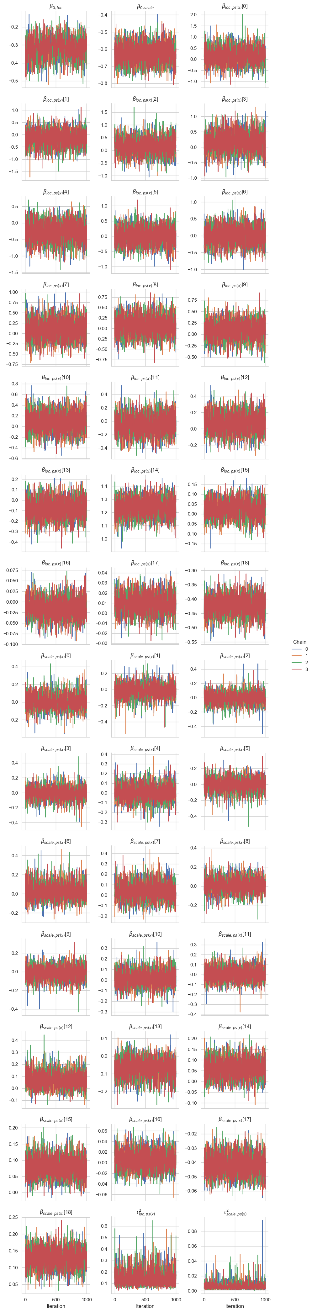
<seaborn.axisgrid.FacetGrid at 0x131f392b0>

Predictions

samples = results.get_posterior_samples()

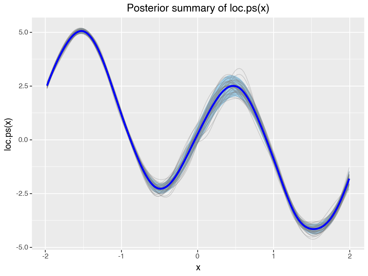
gam.plot_1d_smooth(term=model.vars["loc.ps(x)"], samples=samples)

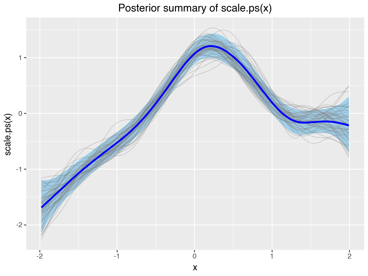
gam.plot_1d_smooth(term=model.vars["scale.ps(x)"], samples=samples)

Predict variables at new x values

x_grid = jnp.linspace(df.x.min(), df.x.max(), 300)

predictions = model.predict(
    samples=samples,
    predict=["loc.ps(x)", "scale.ps(x)", "loc", "scale"],
    newdata={"x": x_grid},
)

predictions_summary = gs.SamplesSummary(predictions).to_dataframe().reset_index()
predictions_summary["x"] = np.tile(x_grid, len(predictions))

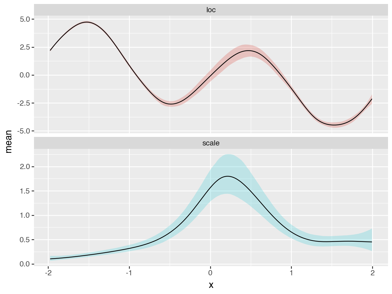
Plot parameters as functions of covariate

select = predictions_summary["variable"].isin(["loc", "scale"])
(
    p9.ggplot(predictions_summary[select])
    + p9.geom_ribbon(
        p9.aes("x", ymin="q_0.05", ymax="q_0.95", fill="variable"), alpha=0.3
    )
    + p9.geom_line(p9.aes("x", "mean"))
    + p9.facet_wrap("~variable", scales="free_y", ncol=1)
    + p9.guides(fill="none")
)

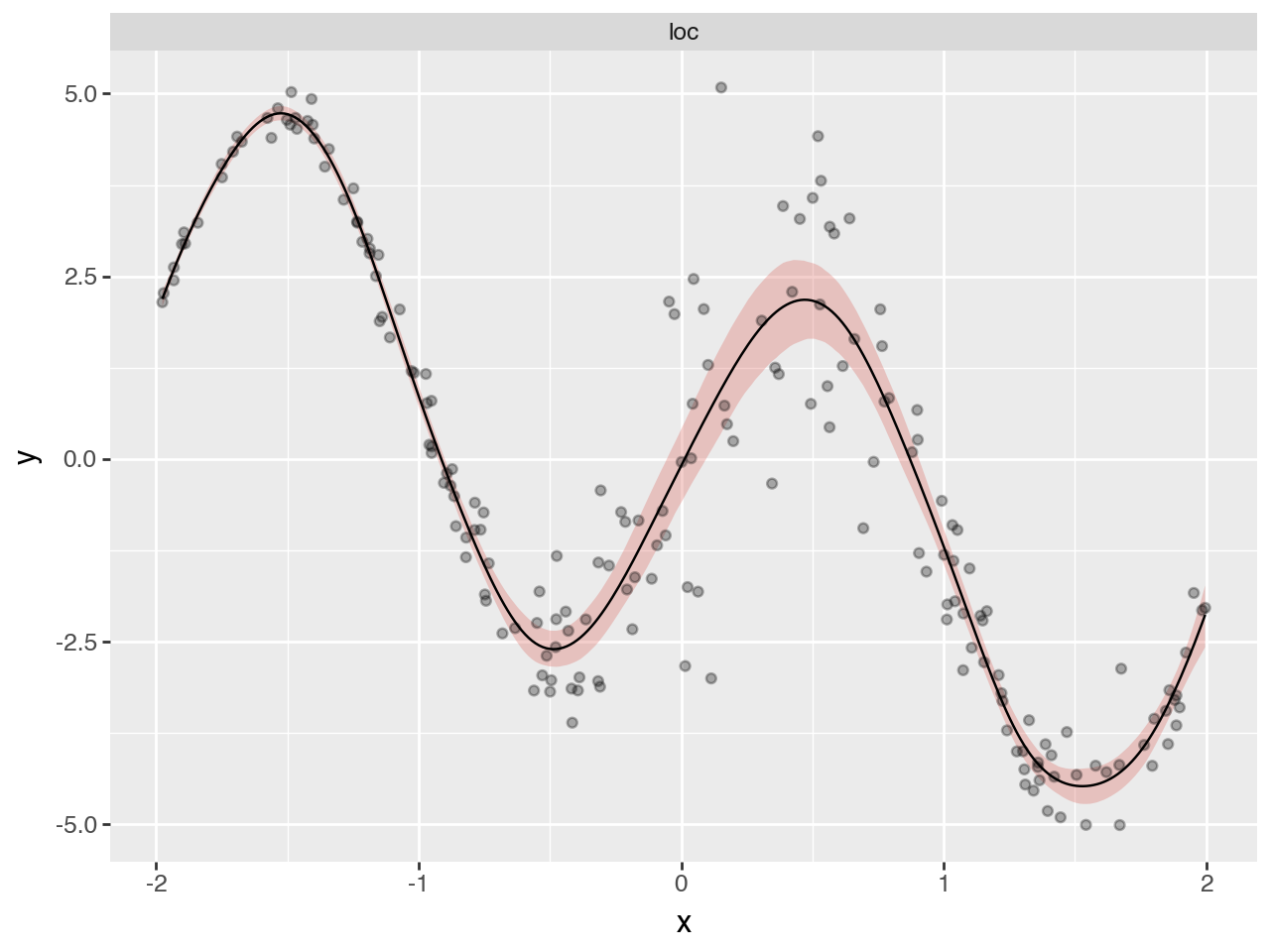
Plot fitted location with raw data

select = predictions_summary["variable"].isin(["loc"])
(
    p9.ggplot(predictions_summary[select])
    + p9.geom_ribbon(
        p9.aes("x", ymin="q_0.05", ymax="q_0.95", fill="variable"), alpha=0.3
    )
    + p9.geom_point(p9.aes("x", "y"), data=df, alpha=0.3)
    + p9.geom_line(p9.aes("x", "mean"))
    + p9.facet_wrap("~variable", scales="free_y", ncol=1)
    + p9.guides(fill="none")
)

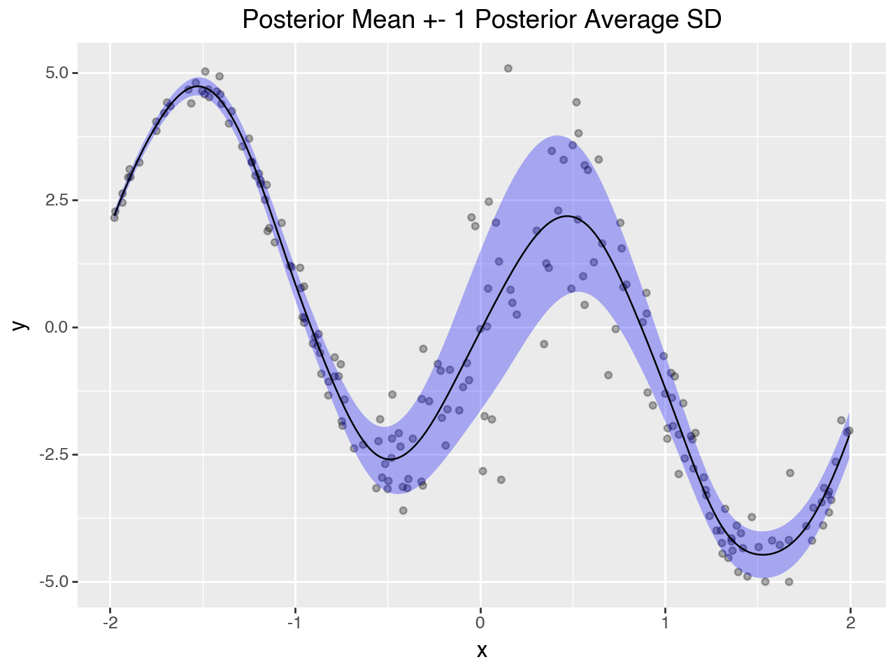
Posterior predictive distribution

select = predictions_summary["variable"].isin(["loc", "scale"])
mu_sigma_df = (
    predictions_summary[select][["variable", "mean", "x"]]
    .pivot(index="x", columns=["variable"], values="mean")
    .reset_index()
)

mu_sigma_df["low"] = mu_sigma_df["loc"] - mu_sigma_df["scale"]
mu_sigma_df["high"] = mu_sigma_df["loc"] + mu_sigma_df["scale"]
mu_sigma_df

variable	x	loc	scale	low	high
0	-1.976702	2.192143	0.102965	2.089178	2.295108
1	-1.963415	2.317238	0.104393	2.212845	2.421630
2	-1.950128	2.439796	0.105870	2.333926	2.545667
3	-1.936841	2.559781	0.107398	2.452383	2.667178
4	-1.923554	2.677188	0.108975	2.568213	2.786163
...	...	...	...	...	...
295	1.942956	-2.635680	0.452966	-3.088646	-2.182714
296	1.956243	-2.513725	0.452268	-2.965993	-2.061456
297	1.969530	-2.388815	0.451673	-2.840488	-1.937142
298	1.982817	-2.261085	0.451194	-2.712279	-1.809891
299	1.996104	-2.130645	0.450848	-2.581493	-1.679797

300 rows × 5 columns

(
    p9.ggplot()
    + p9.geom_point(p9.aes("x", "y"), data=df, alpha=0.3)
    + p9.geom_ribbon(
        p9.aes("x", ymin="low", ymax="high"),
        alpha=0.3,
        fill="blue",
        data=mu_sigma_df,
    )
    + p9.geom_line(p9.aes("x", "loc"), data=mu_sigma_df)
    + p9.labs(title="Posterior Mean +- 1 Posterior Average SD")
    + p9.guides(fill="none")
)

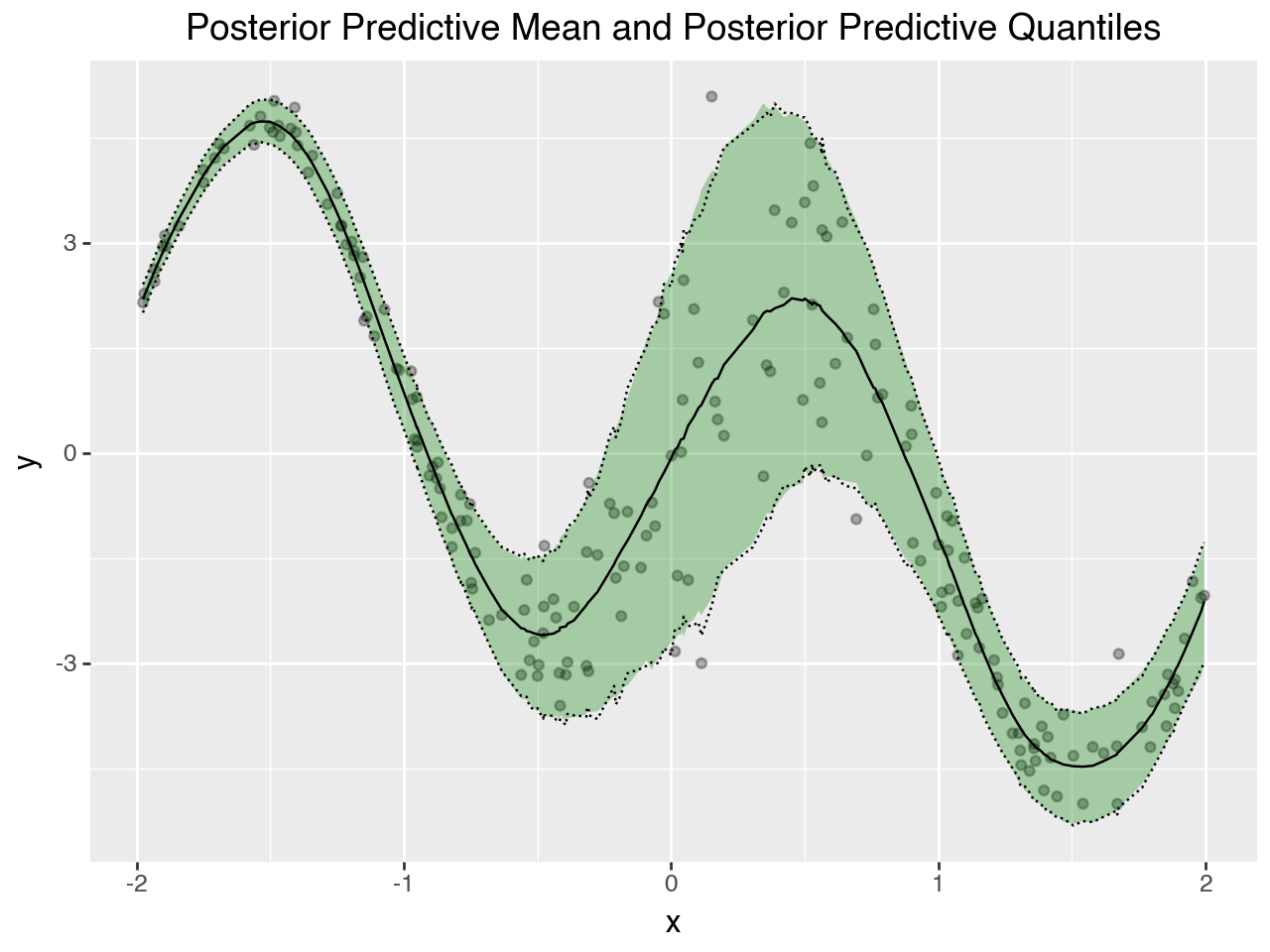
Sample from posterior predictive distribution

import jax

ppsamples = model.sample(shape=(), seed=jax.random.key(1), posterior_samples=samples)

ppsamples["y"].shape

(4, 1000, 200)

# summarise ppsamples
ppsamples_summary = gs.SamplesSummary(ppsamples).to_dataframe().reset_index()

# add covariate to df
ppsamples_summary["x"] = df["x"].to_numpy()

(
    p9.ggplot(ppsamples_summary)
    + p9.geom_point(p9.aes("x", "y"), data=df, alpha=0.3)
    + p9.geom_ribbon(
        p9.aes("x", ymin="q_0.05", ymax="q_0.95"),
        alpha=0.3,
        fill="green",
    )
    + p9.geom_line(p9.aes("x", "hdi_low"), linetype="dotted")
    + p9.geom_line(p9.aes("x", "hdi_high"), linetype="dotted")
    + p9.geom_line(p9.aes("x", "mean"))
    + p9.labs(title="Posterior Predictive Mean and Posterior Predictive Quantiles")
    + p9.guides(fill="none")
)